Weekly maintenance every saturday 03:00 - 06:00 UTC
Backtesting investigation of the effect of the optimized S&P 500 portfolio diversification with $L_2$ regularization.
Introduction.
Modern portfolio theory, or mean-variance analysis, is a mathematical framework for assembling a portfolio of assets such that the expected return is maximized for a given level of risk. It is a formalization and extension of diversification in investing, the idea that owning different kinds of financial assets is less risky than owning only one type. Its key insight is that an asset's risk and return should not be assessed by itself, but by how it contributes to a portfolio's overall risk and return. It uses the variance of asset prices as a proxy for risk. In this model, the return and risk of the stock portfolio are assumed to be the function of the history of the stock marked, namely, the vector of the expected return for stocks $$\mu_i = \mathbf{E} r_i$$ and the covariance matrix for stocks $$ \Sigma_{ij} = \mathbf{E}(r_i - \mathbf{E} r_i) (r_j - \mathbf{E} r_j), $$ where $r_i$ is the historical return for stock $i,$ for some period of time.
The classical Harry Markowitz’s portfolio optimization theory [Mar52]
for long - only portfolio and the minimization of the
portfolio volatility for a given target return could be described as follows:
$$
\begin{array}{ll}
\mbox{minimize} & w^T\Sigma w\\
\mbox{subject to} & w^T \mu \geq \mu^*, \\
& w^T \mathbf{1} = 1, \\
& w \succeq 0.
\end{array} \tag{1}
$$
where a variable to be found, $w$ is the weight (allocation) vector of stocks,
$\mu$ is the expected stock return vector, $\Sigma$ is the estimated stock
covariance matrix, $\mu^*$ is the target portfolio return.
The Markowitz portfolio model with diversification with $L_2$ regularization can be described as follows: $$ \begin{array}{ll} \mbox{minimize} & w^T\Sigma w + \lambda w^T w\\ \mbox{subject to} & w^T \mu \geq \mu^*, \\ & w^T \mathbf{1} = 1, \\ & w \succeq 0. \end{array} \tag{2} $$ where $ \lambda \geq 0$ is the coefficient of $L_2$ regularization, which gives more weights to a stocks, whose weights was small in the calculation result of the previous model. The more the $\lambda$ value, the more the count of stocks with nonzero weight component $w_i,$ the more diversified portfolio we'll get. The other model parameters/variables are the same as in (1).
The backtesting procedure description.
The stock list selection.
The symbol list for S&P 500 was downloaded from wikipedia [SP], there were 505 stocks at the moment. The stock Adjusted Close price data were downloaded for the last 50 years, up to 2021. Then, the stocks with relative NAN count more than $0.4$ were filtered out. The stock count in the filtered price table was about 280 stocks. The earliest date, when the all the columns of stocks have the adjusted close prices without NANs was 1985-08-08. All the records before this date in the stock Adjusted Close price table were cut out. The resulting table was used in the further analysis.
The backtesting.
The dates of test date interval beginning were 15- th day of every month. The backtesting year range was 2002 -- 2019. The date range for the data used for the optimization of the portfolio allocation were in the range from the aforementioned date - 1985-08-08 up to the beginning test interval date. The portfolio optimization was performed with the help of the technique described in [BV04]. The target portfolio return $\mu^*$ was one of $\{0.1, 0.2, 0.25\},$ the coefficient of $L_2$ regularization $\lambda$ was one of $\{0.0, 0.05, 0.1, 0.15\},$ the period of portfolio holding was one year. The averaged portfolio return was calculated as geometric mean of all the portfolio returns for all the months.
The results of backtesting.
Figure 1: Stock count for different portfolio parameters by year.
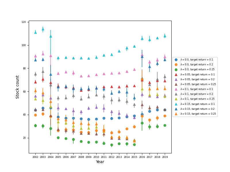
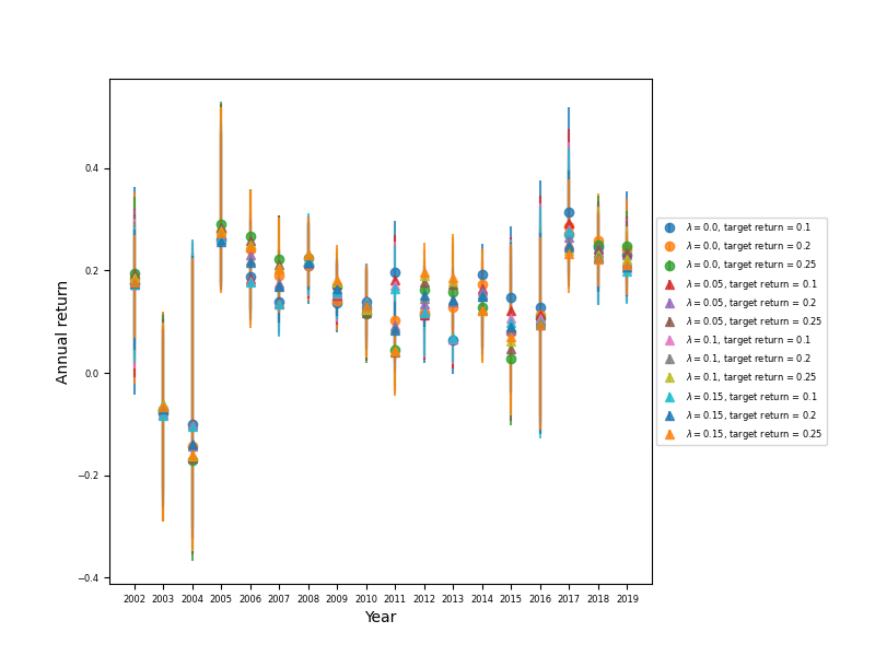
Figure 2: Averaged annual return for different portfolio parameters by year.
The dependency of the portfolio parameters on values $\mu^*$ and $\gamma,$ for the year range 2002 - 2019.
| Target return | $\gamma$ value | Mean stock count | Mean return | Min. return | Max. return |
|---|---|---|---|---|---|
| 0.1 | 0.0 | 39.787 | 0.142 | -0.287 | 0.52 |
| 0.2 | 0.0 | 31.051 | 0.138 | -0.328 | 0.476 |
| 0.25 | 0.0 | 21.87 | 0.136 | -0.367 | 0.53 |
| 0.1 | 0.05 | 65.722 | 0.135 | -0.296 | 0.483 |
| 0.2 | 0.05 | 48.278 | 0.135 | -0.328 | 0.474 |
| 0.25 | 0.05 | 31.333 | 0.136 | -0.355 | 0.525 |
| 0.1 | 0.1 | 81.282 | 0.132 | -0.302 | 0.488 |
| 0.2 | 0.1 | 60.741 | 0.133 | -0.324 | 0.472 |
| 0.25 | 0.1 | 37.407 | 0.136 | -0.348 | 0.519 |
| 0.1 | 0.15 | 98.241 | 0.13 | -0.305 | 0.491 |
| 0.2 | 0.15 | 70.394 | 0.131 | -0.323 | 0.47 |
| 0.25 | 0.15 | 40.912 | 0.135 | -0.344 | 0.518 |
Discussion.
As we can see from the figures and the table, the geometrical average of annual return for year interval 2002 - 2019, was about 0.13 - 0.14 in all the parameter range. It has been exposed, that the mean annual portfolio return for this year range actually nearly not depends on the expected return and the $\gamma$ regularization parameter, if they are changes in aforementioned range, but the minima and the maxima of the annual portfolio return, i.e. the variance of the annual portfolio return, moreover, shows more pronounced dependency on these parameters of the optimized portfolio. The less the expected portfolio return and regularization parameter values, the less the difference between the minima and maxima of the portfolio return for the same $\gamma$ and $\mu^*$ values. The mean portfolio return practically shows no dependency on the expected portfolio return, that could be due to the heteroscedasticity of a stock market. Also, the diversification of the optimized portfolio causes the portfolio variance to increase, that can be assumed as an undesirable effect.
References:
[BV04]
S. Boyd and L. Vandenberghe. Convex Optimization. Cambridge University Press,
2004.
[Mar52] H Markowitz. Portfolio selection. The Journal of Finance, 7(1):77––91, 1952.
[SP]
List of sp 500 companies.
https://en.wikipedia.org/wiki/List_of_S%26P_500